This page is dedicated to describe in detail how to use and run hpocket server. For several reasons, two servers are available to run hpocket:

• Default server
• Advanced server (Mobyle)

In this page, you will find detailed documentation on how to run hpocket for both servers (input & output).

To run hpocket, you need a query protein sequence, either under the form of a PDB file (hpocket will only consider the amino-acids sequence, not the coordinates), or a fasta sequence. You can also control the Blast parameters that will retrieve homologous structures. The following section will describe how to run hpocket on both server.

Default server

Running a hpocket job

1. Browse (2) your local hard drive to provide a PDB file,or directly paste (1) your multiple PDB file in the text area.
2. Alternatively, you can enter a fasta sequence by browsing your hard drive or pasting your data in the appropriate form.
    
   
3. Optionally, you can change the default value of several Blast parameters, eg. the E-value threeshold (a), the maximum number of homologous structures to retrieve (b), and the minimum sequence coverage percentage (c).
    
   
4. Optionally, enter your email (3) to be notified when your job will be finished.
5. Once your data have been entered properly, you will have to enter the word shown in the captcha image (4). This is to avoid automatic programs to do nasty stuffs with our server.
6. You can now run hpocket by clicking on the Submit button (GO!). Clicking on the clear button will clear all input data you entered.

Alternatively, you can test the server, using inhouse demonstration data. To do so, just check the Demo checkbox shown in the picture bellow, and go to step 3 (any input data will be discarded then).

Note that you can give a name to your job using the following text field. The default name contains the service name plus the current date and time.

<Back to top>

Intermediate page (job status)

Once you have submitted your data, a new job will be created. You will be redirected to an intermediate page. From there, you just have to wait the end of your job, or bookmark the result page using the adress given in this page. Then, when your job will be finished, you will have a new intermediate page, from where you will have to click on the provided link to obtain the results page described in the output results section.

<Back to top>

Advanced server (Mobyle)

Running hpocket job

To run hpocket using Mobyle, you need to provide the same input types as described for the default server. The only difference is the interface, and that you have the possibility to retrieve PDBs directly from the Protein Data Bank database.

Here is a short description of the mobyle interface:

1. Provide your PDB structure by using the first form labeled Query PDB (PDB), shown in the snapshots bellow. You have 3 possibilities to enter your data, each of these being selected by clicking on the corresponding radio button:
   1. Copy/paste (1): Simply copy and paste your PDB data in the text area.
   2. Database (2): Select your database using the combo box (a), and enter a valid PDB 4 letter code (b).
   3. Local file (b): Select a local file stored on your computer.
   
    
2. Alternatively, you can enter a fasta sequence in the appropriate form. Follow the exact same procedure as the one described for PDB, but instead use fasta sequences (and available sequence databases).
3. Optionally, you can change the default value of several Blast parameters, eg. the E-value threeshold (a), the maximum number of homologous structures to retrieve (b), and the minimum sequence coverage percentage (c).
4. You can now run fpocket by clicking on the Run button (GO!). Clicking on the Reset button will clear all input data you entered
5. The first time you will run hpocket, you will have to enter a security string. Don't worry, you only have to do this the first time you run hpocket.

You can also test the server by using inhouse demonstration data. To do so, just check the Demo checkbox shown in the picture bellow, and go to set 3 directly (any input data will be discarded then).

Note that you can also give a name to your job using the following text field.

Intermediate page (job status)

Once you have submitted your data, a new job will be created, and you will be redirected to this new job tab page as shown bellow. From here, you just have to wait for results to appear.

<Back to top>

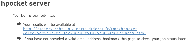
We use the same output page to display results of hpocket job for both server. Before describing it, we just describe for both servers, how to reach this page. Don't worry it's really easy.

Getting to the results page

Default server

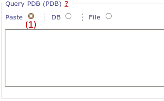
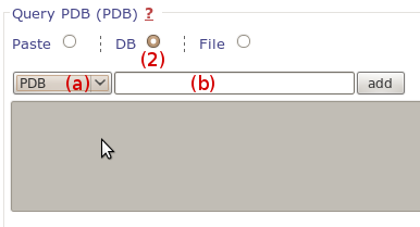
Just follow the input tutorial, where we describe all intermediates pages from which you will be able to reach the results final page.

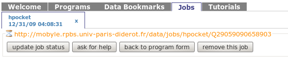
Advanced server (Mobyle)

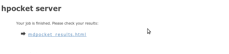
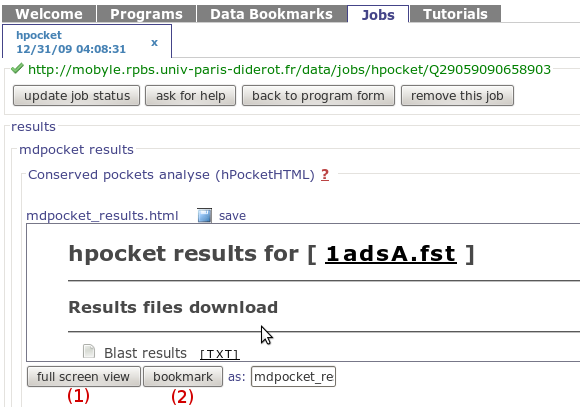
In mobyle, once your job will be finished, you will be redirected to the mobyle results page. This results page is shown in the snapshot on the right. The results page is actually contained in the "Conserved pockets analyse alpha spheres (hpocket HTML)" labeled scroll pane. To have a more friendly view and reach the output pages described just click on the Full screen view button (1)

You also have the possibility to bookmark the result page using the Bookmark button (2) (enter the bookmark name in the field on left)

Note that main program output results are provided both in the final results page and in the mobyle interface. This redundancy is comfortable to (i) analyse your results in a specific and integrated web page and (ii) to directly use the mobyle pipelining feature for further analysis.

<Back to top>

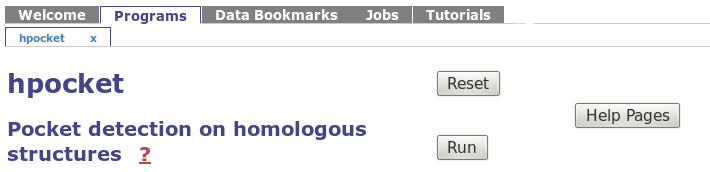
Results page description

The results can be roughly divided in 3 sections: output files, snapshots and Visualisation.

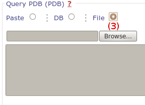
Output files

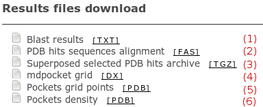
Several hpocket output files are provided and described bellow. You can download all of them.

• Blast results (1): a text report for blast search.
• PDB hits sequence aligment (2): a fasta file containing aligned homologous sequences
• Superposed selected PDB hits archive (3): an archive containing all superposed homologous structures (PDB).
• mdpocket grid (4): it is the mdpocket output grid that stores density information for each grid point. To learn more about hpocket methodology and output, go tho the hpocket method section in the homepage, or read the documentation.
• Pockets grid point (5): This file contains all grid points having 3 or more Voronoi Vertices in the 8A3 volume around the grid point for each homologous hit. This output should be used to define a specific zone (a pocket) on which you may want to make further analysis using mdpocket (not available in the hpocket server though, you will have to run it yourself using the desktop package).
• Pocket density (6): This file contains the query protein, written as PDB file, with the B-Factor values representing alpha spheres density. Such a file allows intuitive, coloured visualisation similar to that of the snapshots described below.

<Back to top>

Snapshots

Two set of snapshots are provided here: the first set (left picture) represents the superposition of all retrieved homologous structures, and the second set (right picture) represents the query structure surface coloured by alpha spheres density. Here, coulours range fromblue (low density = no particular cavity at this place) to red (high density = hot spot = conserved cavity!).

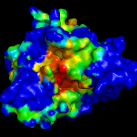
Note that you may obtain such display by dowloading output PDB file "Pocket density" described previously, and display it using pymol and VMD (color the molecular surface by Bfactor).

<Back to top>

Visualisation

Currently, the visualisation is made using both Jmol and OpenAstex, in which the mdpocket output PDB file is automatically loaded in each viewer (1) (query protein).

Using Jmol, you can view the Grid file extracted from mdpocket results. A slider is provided to change isovalue: the highest the isovalue is, the more conserved is the corresponding cavity.
Using OpenAstex, the visualisation is atom-centered. That is, the isovalues have been mapped from the grid to the atoms and transformed to be somehow B-factor-like for coloring purposes. The highest the B-factor is, the more conserved is the cavity associated with atoms.

Both visualisation methods use different metrics. Isovalues will tipically range from 0 to N, with N having no real limitation (depends on the number of snapshots; the slider is limited to 800), while B-factor will range from 0 to 7-8, as it is log-scaled. We are investingating a way to get a common metric, and to merge these visualisation features in a single viewer.

Jmol

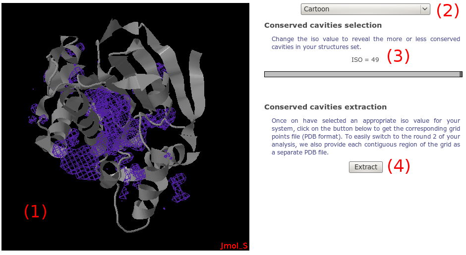
Using Jmol, the density grid is loaded along with the protein (1). On the right, you have a set of graphic components to facilitate the viewing. A simple selection box (2) allows you to perform basic changes to the whole system representation (display protein as cartoon, reset view...).

Using the slider on the right, you can change (3) the so called "isovalue". For a given grid point, this isovalue represents the number of alpha spheres seen for all snapshots within a 8A radius. Thus, a high isovalue will display protein cavities which are highly conserved among homologous structures, while low isovalues will rather show these conserved zones plus other less conserved zones, which might be pockets specific to one or several proteins.

As for mdpocket, we give you the opportunity to downlad grid points (PDB format) corresponding to each contigous points that could form a potential pocket(4). As there is no point to run the second round of mdpocket to homologous structures, you may use these files only to check how and where the conserved or transiant zones are located on each homologous structures.

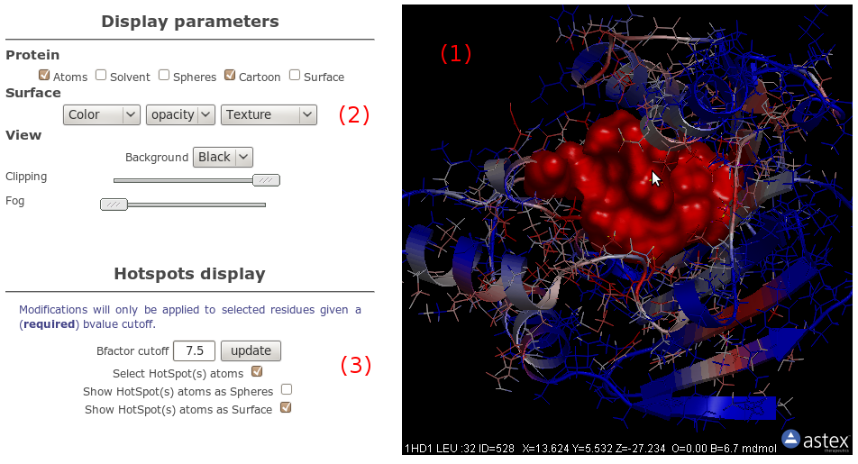
OpenAstexViewer

Using OpenAstex, atoms are coloured by B-factor, with the same convention as that used for snapshots, that is, the more an atom is close to red (resp. blue), the more conserved is its corresponding cavity. Only here, the grid isovalue have been mapped on atoms (see accompagning paper for formula) so you can see directely which atom is associated with a conserved zone. In other words, red atoms may be part of common cavities among homologous, while blue atoms may be part of specific (or inexistant) cavities.

Besides basic visualisation options (2), we give you the possibility to select atoms based on B-factor value (3). By checking the appropriate checkbox, all atoms having B-factor up to the specifiede value (in the text field) will be selected. If you change this isovalue cutoff, you have to click the update button to update atom selection. 0 is the minimum B-factor value, while the maximum should lie around 7 or 8 (due to log-scaling of isovalues).

Remember that if you know Jmol and OpenAstex, you can access the display popup menu by right clicking on the view.